Python KNN Algorithm And Sample Application
Hello;
In this paper we will talk about the closest neighbor(knn / K neighborhood) algorithm used in classification technique. The narrative be clear on behalf of a class attribute to a certain value, for example, the particular value of the class attribute when we talk about the guy I’ll tell him.

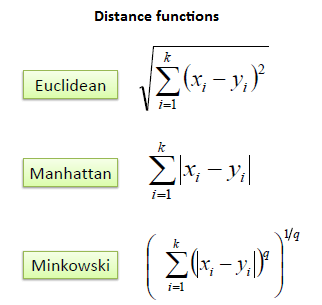
Knn algorithm; (in the space formed by the elements which have the class attribute set to a new instance (of the class nature non-specific) added to this when, for example, an algorithm that determines whether it should be included in the closest class. It uses a k variable to determine the class closest to it. This variable K represents the number of elements that are closest to the instance. The following 3 distance functions are commonly used when calculating the distance between the elements.
Euclidean function is a function that we have been familiar with since elementary school or high school. In fact, don’t be afraid of your eyes, all derived from one main function. We get the form of the Manhattan distance for the value q=1 in Minkowski, and the Euclidean distance for the value q=2. Therefore, we will use minkowski’s general formula to implement. Thus, the person will only change the Q value for other distance measurements.
If we summarize the algorithm with a few items;
- Add a new instance to a space made up of elements with class attributes.
- Set the K count.
- Calculate the distance between the new sample and the elements.(Using one of the offset functions))
- Look at the class attribute of the closest K element.
- Include an instance of the class whose class value is greater than the number of elements that are closest to it.–
Learn KNN Algorithm Python
The theoretical part of the algorithm ends here. Now let’s do both practice and practice with Python. As you know, the first thing we need is an appropriate data. We’re going to use the data set here for the application we’re going to do. In this data set, the color values(r, g, b) of the human face (SIMA) in pictures of people of different ages,sexes,races are taken. There are also non-human face samples from the color values in the dataset. As a result of these values taken 4. in milk, this value is 1 if it belongs to a human face, if not we have a class that holds a value of 2 which is. Because our data set is too large, we will only use a fraction of the data set because our personal computers will be forced to process it(at least mine). Since the class separation in the data set starts at 50.859 lines, we will read the data set considering this information. Although it is a bit easier to parse the data set with libraries like pandas, we will not use any Library for the parse process in this application. I thought it would be better to share the code as a whole rather than share the part and make the necessary comment.
1 2 3 4 5 6 7 8 9 10 11 12 13 14 15 16 17 18 19 20 21 22 23 24 25 26 27 28 29 30 31 32 33 34 35 36 37 38 39 40 41 42 43 44 45 46 47 48 49 50 51 52 53 54 55 56 57 58 59 60 61 62 63 64 65 66 67 68 69 70 71 72 73 74 75 76 77 78 79 80 81 82 83 84 85 86 87 88 89 90 91 92 93 94 95 96 97 98 99 100 101 102 103 104 105 | #!python3 #50859 (Class id) # Libraries for graphics. Axes3d for a 3D graphics. from matplotlib import pyplot as plt from mpl_toolkits.mplot3d import Axes3D class knn(): our startup function and variables. INP variable class qualification # it's our obvious example. You can also get this value from the outside if you want. # _init _ _ method dataset data set, K closest neighbor, nfrom data # set the row and begin to read the line which he would read until the nto # specifies. The last two parameters are sufficient for PCs when analyzing large sets of data * you can optionally only part of the data set # I added it to choose Which is an example in our example. def __init__(self, dataset, k, nfrom, nto): self.b, self.g, self.r, self.class_attr = [], [], [], [] self.inp = [264,124,183] self.k = k # We read our data set from the nfrom line to the nto line. # We also add each column in the data set to a list. (r,g,b, class_attr) with open(dataset, "r") as f: for i in f.readlines()[nfrom:nto]: self.r.append(int(i.split()[0])) self.g.append(int(i.split()[1])) self.b.append(int(i.split()[2])) self.class_attr.append(i.split()[3]) Our method of calculating distance according to the dist parameter # related calculation is performed . Default oklid distance is used. # The most important point to note here is that the distance value is calculated # then we don't know which offset is the index number at first. # Because we will use this index number to reach the class value of the respective offset. # For this reason, The distance and distance index value in a bunch # we add it to our dist list.Because when we sort the distance from small to Big # we can't reach the actual class value of the distance. def distance(self, dist=1): self.dist = [] #operations such as exponent, absolute value, such as mixed for loop #the minkowski formula is the equivalent. for i in range(len(self.class_attr)): self.dist.append((pow((pow(( abs(int(self.b[i]) - int(self.inp[0])) + abs(int(self.g[i]) - int(self.inp[1])) + abs(int(self.r[i]) - int(self.inp[2]))), 2)), 1/dist), i)) return self.dist # K which is closest to our example after calculating the distance # we find the element and class values of these elements class_values # we keep it on our list And 1 in the class_values list of the loop) # 2(Not volume) calculate the number of numbers, for example, which class belongs to we find it. def findClass(self): self.class_values = [] self.result = "" for i in sorted(self.dist)[:self.k]: self.class_values.append(self.class_attr[i[1]]) self.first = self.class_values.count("1") self.secnd = self.class_values.count("2") print("Birinci Sınıf:", self.first) print("İkinci Sınıf:", self.secnd) if self.first > self.secnd: self.result = "1. Sınıf(Kırmızı)" else: self.result = "2. Sınıf(Yeşil)" print("SONUÇ: "+self.result) #Visualization # In 3D space for a more concrete understanding of the algorithm # create graph. Red spots skin, green spots skin # and the blue dot is our example of class value that is not clear. def grafik(self): fig = plt.figure() ax = fig.add_subplot(111, projection='3d') for bi, gj, rk, class_attr in zip(self.b, self.g, self.r, self.class_attr): if class_attr == "1": ax.scatter(bi,gj,rk, c='r', marker='.') else: ax.scatter(bi,gj,rk, c='g', marker='.') ax.scatter(int(self.inp[0]), int(self.inp[1]), int(self.inp[2]), c='b') ax.set_xlabel('X Ekseni') ax.set_ylabel('Y Ekseni') ax.set_zlabel('Z Ekseni') fig.text(0, 0, "Kırmızı(1)[Cilt] : "+str(self.first)+ " -- Yeşil(2)[Cilt Değil] : "+str(self.secnd)+ " -- {{SONUÇ : "+self.result+"}}") plt.legend() plt.show() ins = knn("ten_dataset.txt", 17, 50300, 51000) ins.distance(1) ins.findClass() ins.grafik() |
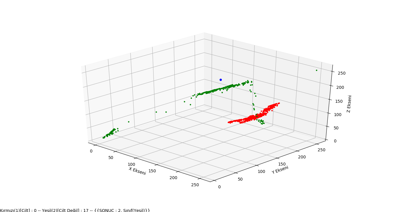
The view of our application in 3D space is as follows. Our blue dot example(class is not certain), red dots represent the skin(SIMA) class, and green dots represent the non-skin class. As you can see clearly in the graph, our example is included in the class closest to it by our application.

